Home Page
We prepare the next generation of problem solvers to discover and innovate solutions for the future.
The College of Science promotes novel ways of thinking and implementation in a rapidly changing world.
We provide our scholars with hands-on experience, cross/multi-disciplinary research, and faculty and staff mentors who not only educate but inspire our scholars.

Join us for Fall 2026
There's still time to apply. For some programs, applications will be reviewed on a rolling, space-available basis.

Join Us for Accepted Student Open House
Visit campus on March 28 or April 11 to meet faculty, tour campus, and ask your questions.


Faces of RIT
-
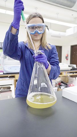
Medicine's Future
Nicole PannulloBiochemistryBy working on a faculty-guided research project, Pannullo has gained hands-on research experience to pursue a future in regenerative medicine. It’s one way Pannullo is putting experiential learning to work.
-
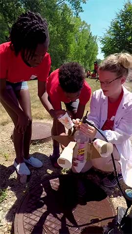
Connecting Kids to Science
Devon M ChristmanPhysicsOver the summer, Christman taught a workshop called “Experiments in Science” to a group of children from RIT’s Kids on Campus program. By helping to change their perspectives on who and what a scientist is, Christman is shaping the minds of tomorrow’s scientists.
-
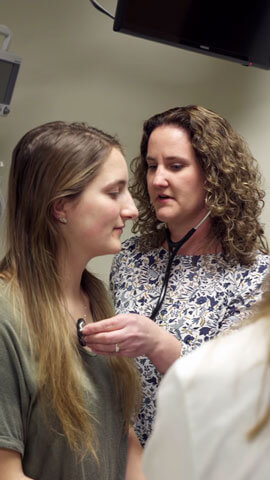
Giving Back
Jennifer Wheeler, M.D. BS ’01BiotechnologyFamily MedicineAfter 9/11, Wheeler enlisted in the US Army and served as a doctor in Afghanistan. Now, she practices family medicine and serves as a preceptor to RIT students who are embarking on their own careers in medicine.
-
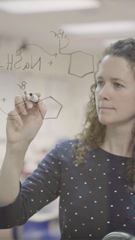
Expanding ASL
Tina Goudreau CollisonProfessor of ChemistryA complicated vocabulary and a lack of dedicated signs in American Sign Language makes Organic Chemistry a challenge for deaf and hard of hearing students. Collison worked with interpreters to develop new ASL signs, leading to profound learning improvements for her students.
-
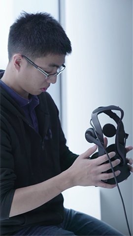
Enhancing Reality
Kevin KhaImaging ScienceKha interned with Oculus testing their next generation of VR cameras, which have the potential to aid law enforcement and impact learning in schools. The internship turned into a full-time job, and Kha plans to work on enhancing the VR experience.
Latest News
-
March 9, 2026

RIT sets course for the future with 2035 Strategic Framework
RIT has launched a new decade-long strategic framework that will guide the university’s priorities, investments, inspiration, and aspirations through 2035.
-
March 5, 2026

Researchers are combining drones and AI to make removing land mines faster and safer
In an article for The Conversation, imaging science Ph.D. student Sagar Lekhak explains how using drones, sensor data, and AI can make detecting land mines safer and more efficient.
-
February 18, 2026

Ph.D. student recognized for work in optics
Imaging science Ph.D. student Muhammad Akif Qadeer has been awarded the 2025 Harvey M. Pollicove Memorial Scholarship from the Optica Foundation. The award is given to one student each year who shows potential in precision optics manufacturing and lens design.
-
February 11, 2026

Imaging science Ph.D. student advances photo conservation
Imaging science Ph.D. student Diane Knauf is shining new light on old images with help from a grant from the National Park Service.
