Development of Science Traceability Matrices for LandIS

The Landsat Next Instrument Suite (LandIS) is committed to extend the nearly fifty-year data record of spaceborne measurements of the Earth’s surface collected from Landsat’s reflective and thermal instruments. The goal of the LandIS mission is to continue the mission of the Landsat program for acquisition, archival, and distribution of imagery to characterize decadal changes in the Earth’s surface. LandIS will consist of a constellation of three satellites, which will provide an improved temporal revisit (a six-day revisit) for the purpose of monitoring dynamic changes in the Earth’s surface. The sensor will also be a significant change in the number of spectral bands compared to its predecessors - Landsat 8/9 - which currently consists of 11 spectral bands at 30-m GSD. While, LandIS will have a total of 26 spectral bands at Ground Sample Distance (GSD) of 10-m, 20-m and 60-m. This will result in a significantly higher data volume compared to its predecessor. This increase in data will require a more efficient compression algorithm currently being implemented for L9; a lossless compression algorithm based on the Consultative Committee for Space Data Systems (CCSDS) 121.0 recommendation standard. After exploring available options, CCSDS-123.0 B2 emerged as the top choice. This open compression standard provides high-performance lossless and near-lossless compression, crucial for maintaining data integrity in scientific applications. 

Project Status: LandIS will collect imagery in five LWIR bands, compared to the two thermal bands available on Landsat 8 and 9. This expanded capability enables the derivation of both surface temperature and emissivity. We examined how near-lossless compression might influence the accuracy of Level 2 surface temperature (ST) retrieval using the Temperature and Emissivity Separation (TES) algorithm. DIRSIG was used to simulate LWIR scenes. For this initial study, two thermal DIRSIG scenes were created—Rochester and Idaho—each covering a 30 km × 30 km area at a 60 m ground sample distance (GSD).

The radiometric governing equation in the long-wave infrared (LWIR) region is as below:
$L_TOA = L(T_s)ετ + (1-ε)τL_(↓) + L_(↑)$ [1]

The equation includes top-of-atmosphere radiance (L_TOA), surface radiance (L(T_s)), emissivity (ε), transmission (τ), downwelling radiance (L_(↓ )) and upwelling radiance (L_(↑ )). Surface emissivity and temperature are input parameters for DIRSIG to model the top-of-atmosphere radiance. The atmospheric components—downwelling radiance, upwelling radiance, and transmission—are calculated using the MODTRAN radiative transfer model.

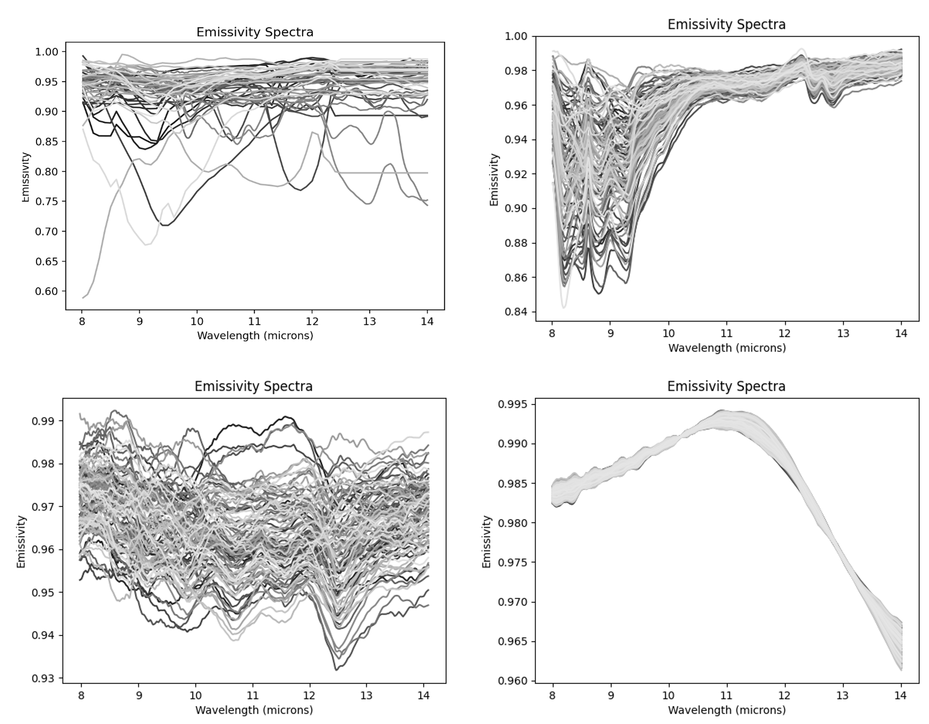
Figure 1: Emissivity database used as an input to DIRSIG. Total of 350 spectral across four materials: Man-made, soil, vegetation, and water.

The DIRSIG simulation ingests different inputs, namely: temperature map, emissivity database, class map, and texture map. Landsat B10 ST product at 30-m GSD was used as the temperature map. The emissivity database is a combination of UCSB and ECOSTRESS datasets in the 8–14 μm region, comprising 350 spectral profiles across four classes; see Figure 1. For the class map, a combination of ESA land cover map at 10-m GSD and a manual classification was used. The texture map took advantage of ASTER GED bands 10–14 at 30-m GSD. Texture map derives the procedure to sample spectra from the emissivity data base. Figure 2 illustrates the inputs and the generated outputs from DIRSIG for a simulated scene in Rochester.

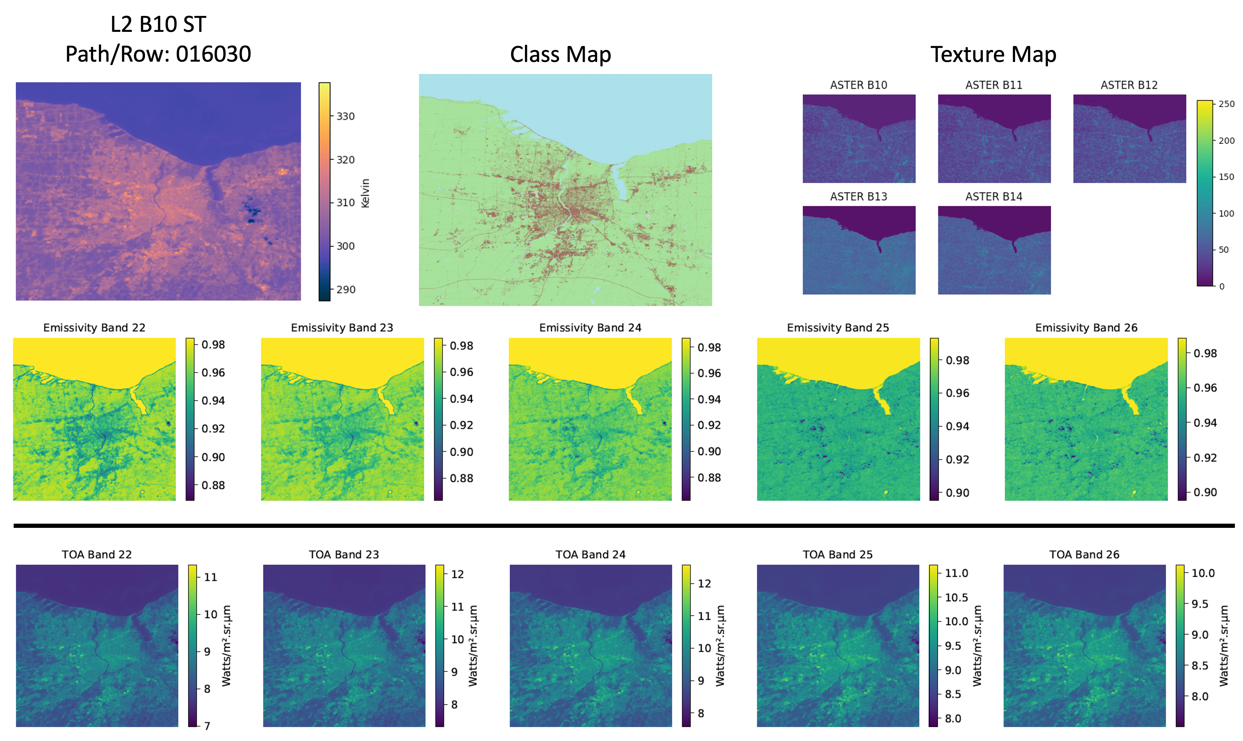
Figure 2: Inputs and outputs to DIRSIG for thermal simulation of five Landsat Next thermal bands. The outputs from the simulation are also used to retrieve error budgets.

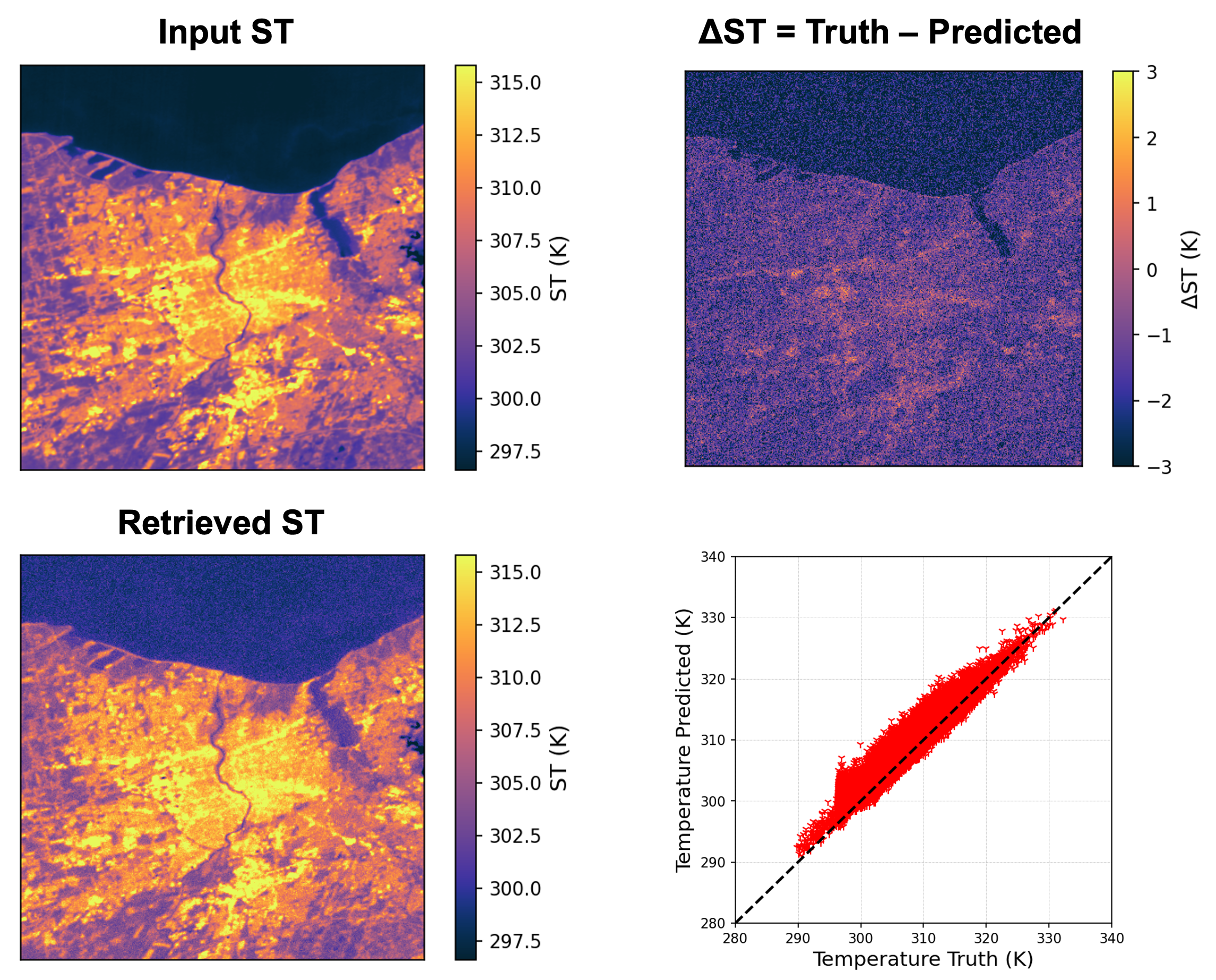
Figure 3: (a) The input surface temperature (ST) used to simulate the LWIR image over Rochester. (b) The retrieved ST using the TES algorithm, incorporating four different sources of uncertainty modeled in the DIRSIG scene. (c) The difference image between the input and retrieved ST. (d) A plot of the input ST versus the retrieved ST, including the 1:1 line for comparison.

We aimed to use the proxy-LandIS dataset created in the LWIR to develop an error budget for the Level 2 surface temperature product, focusing specifically on the error introduced by compression. The primary sources of uncertainty in deriving surface temperature for LandIS include: (1) algorithm error, (2) signal noise (NEDT), (3) absolute radiometric uncertainty, (4) atmospheric error, and (5) near-lossless compression. Figure 3 illustrates the impact of these four uncertainties on the retrieval of surface temperature. Figure 3a shows the input ST from DIRSIG, while Figure 3b presents the ST retrieved using the TES algorithm. Figure 3c displays the difference image between the input and retrieved ST, and Figure 3d provides a plot of the input ST versus the retrieved ST, along with the 1:1 line for comparison.

The errors associated with each component are summarized in Table 1. The total error in the retrieved surface temperature (ST) product was 2.079 K. The largest source of uncertainty was atmospheric uncertainty (1.615 K), followed closely by absolute radiometric uncertainty (1.604 K). While near-lossless compression had the smallest impact (0.098 K). These finding highlights that near-lossless compression is a viable option for data storage and transmission, as it does not compromise the quality of the Level 2 ST product. This trend was consistent across different scenes, including the Idaho scene, where similar results were observed.

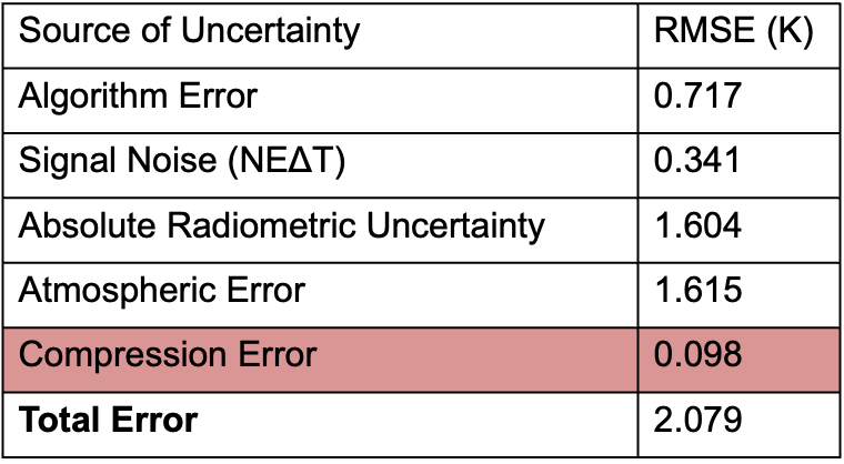
Table 1: The error budget in deriving ST from the modeled DIRSIG scene due to the following sources of uncertainties: (1) algorithm error, (2) signal noise (NEDT), (3) absolute radiometric uncertainty, (4) atmospheric error, and (5) near-lossless compression.